卷积神经网络(CNN)
卷积神经网络CNN(Current Neural Network)与普通神经网络类似,它们都有可学习的权重(Weights)和偏置常量(biases)的神经元组成。每个神经元都接受一些输入,并做一些点积计算,输出是每个分类的分数,因此,普通神经网络里的一些计算技巧在CNN中依旧适用。CNN常用于计算机图像识别。
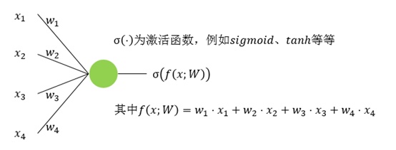
- 普通神经网络:
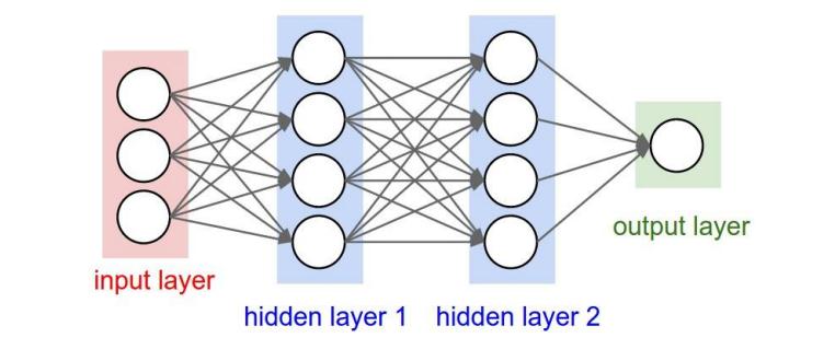
- 卷积神经网络:
卷积神经网络默认输入是图像,可以让我们把特定的性质编码编入网络结构。另外,卷积神经网络是具有三维体积的神经元。
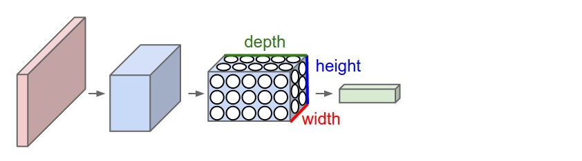
卷积神经网络利用输入是图片的特点,把神经元设计成三个维度:width,depth,height(ps:depth不是神经网络的深度,用来描述神经元的)。
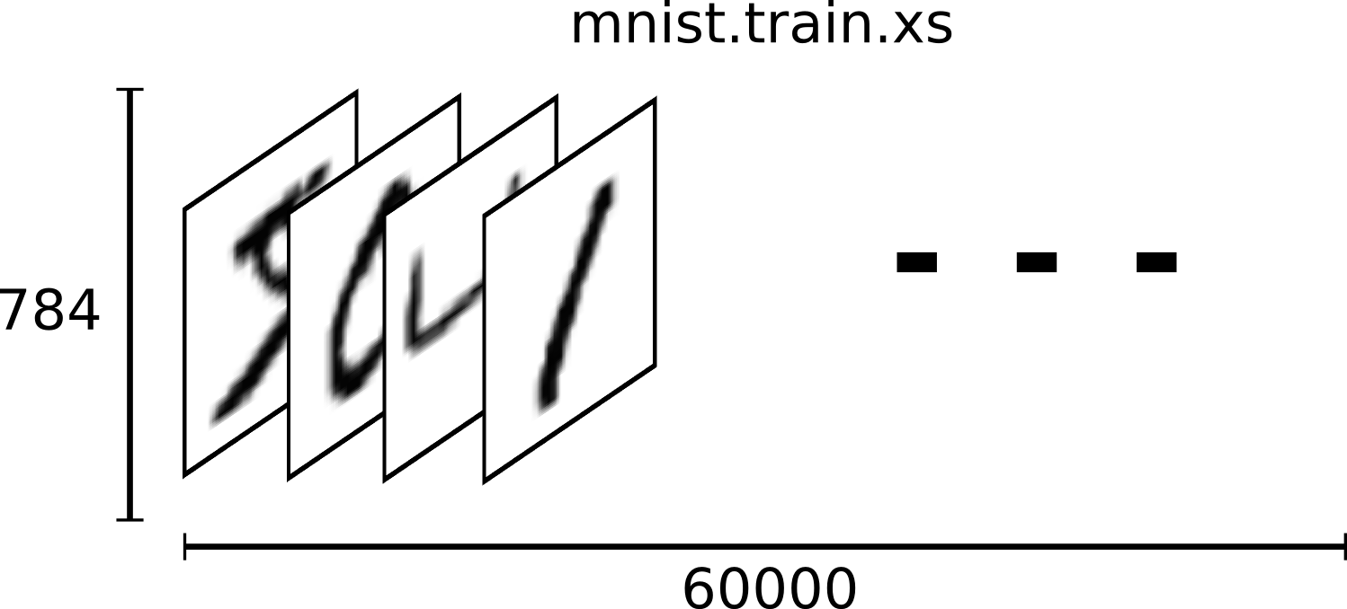
比如输入的图片大小是32323(RGB),那么输入神经元也具有32323的维度
总结:
一个卷积神经网络由很多层组成,输入时三维的,输出也是三维的,有的层有参数,有的层不需要参数
卷积神经网络的组成
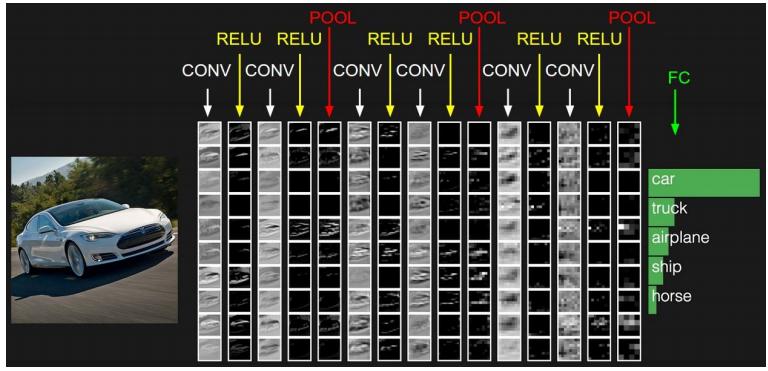
- 卷积层(Convolutional layer):CNN中每层卷积层由若干卷积单元组成,每个卷积单元的参数通过反向传播算法优化得到的。卷积运算的目的是提取输入的不同特征,第一层卷积可能只能提取一些低级的特征比如边缘、线条、角等层级,更多层的网络能从低级特征中迭代提取更复杂的特征。
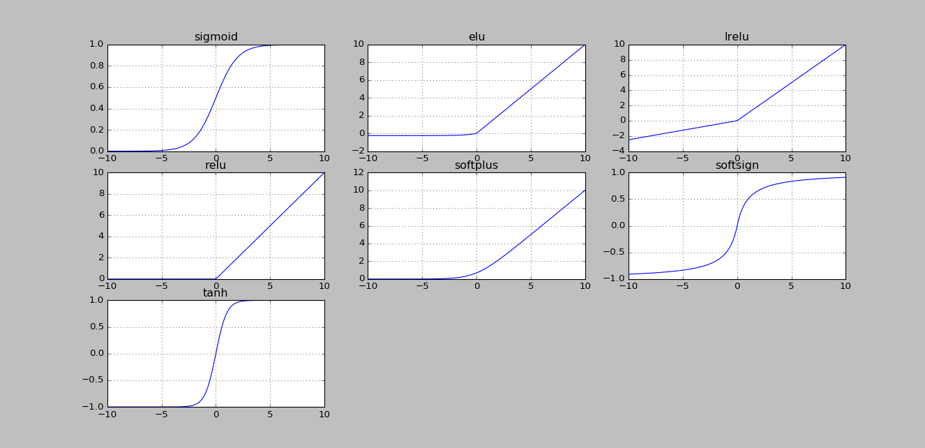
- 线性整流层(Rectified Linear Units layer,ReLU layer):这一层是激励函数(Activation Function),使用线性整流(Rectified Linear Units,ReLU)
- 池化层(Pooling layer):通常在卷积层之后会得到维度很大的特征,将特征切成几个区域,取到最大值或者平均值,得到新的,维度较小的特征。
- 全连接层(Fully-Connected layer):把所有局部特征结合变成全局特征,用来计算最后每一类的得分。
卷积神经网络的过程:
CNN的个人理解
- CNN专门解决图像问题的,可以把它看做特征提取层,让在输入层上,最后用MLP做分类。
- CNNs相对于MLP(Multi-Layer Perceptron,多层感知器,是最简单的DNN),多了一个先验知识,也就是数据之间存在空间相关性。就比如图像、蓝天附近的像素点是白云的概率会大于是汽车的概率。滤波器filter会扫描整张图像,在扫描的过程中,参数共享。
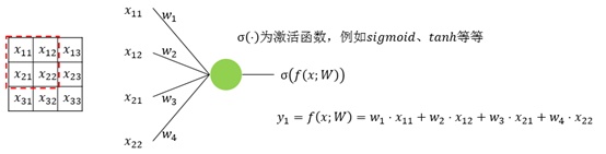
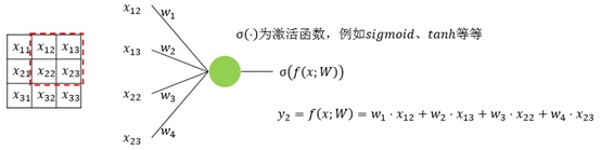
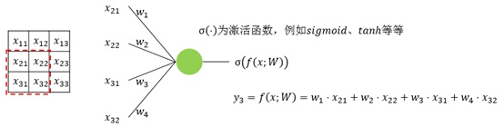
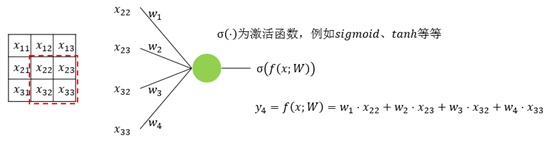
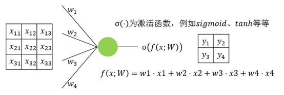
上面4附图,都是一个33的输入经过一个22的conv卷积层的过程。该卷积层conv的strides是1,padding为0
注:参数strides,padding分别决定了卷积conv操作中滑动步长和图像边沿填充方式。
- 输出的结果为:
卷积的理解
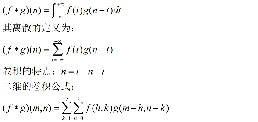
学过概率论都知道有卷积公式吧。
- 卷积公式: