Autoencoder自编码
1 | #author:victor |
运行结果:
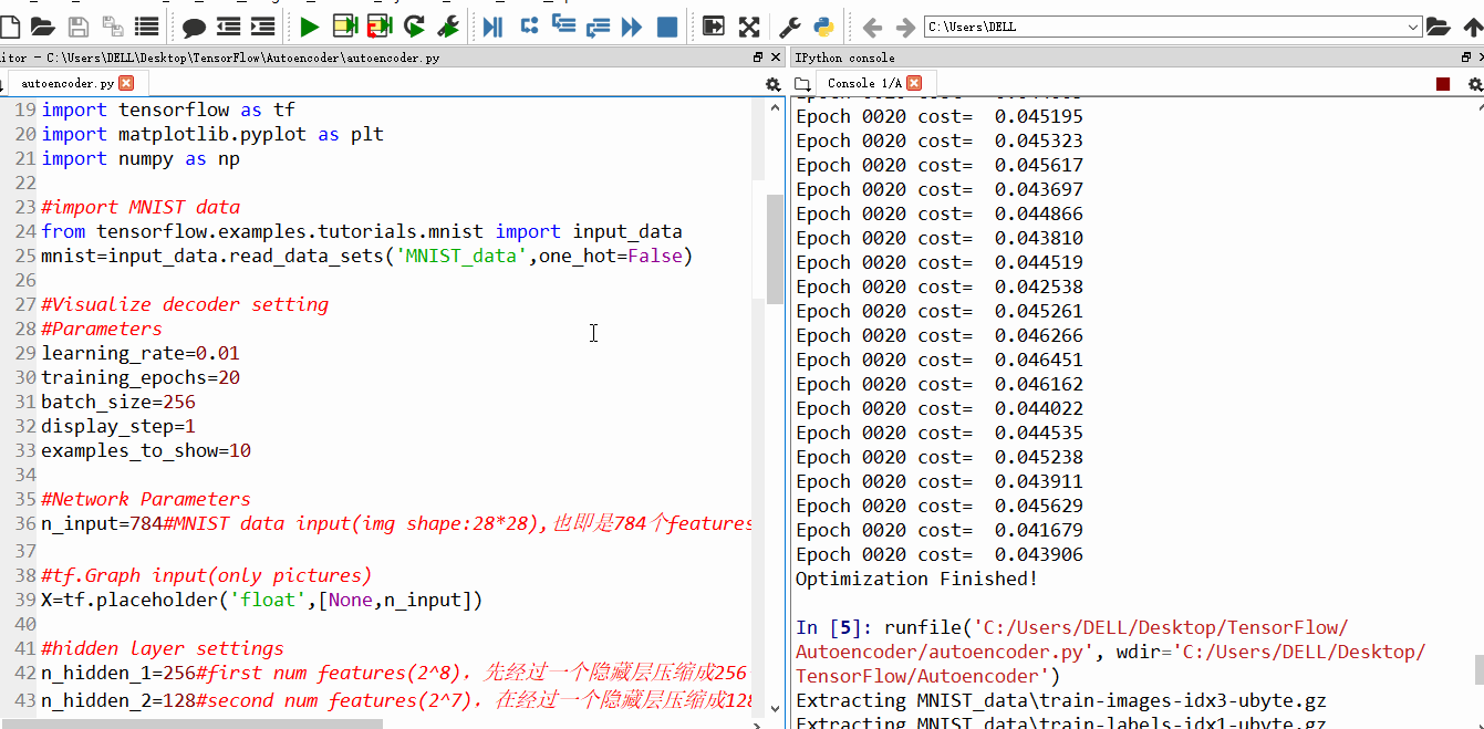
总结:发现经过压缩过后的MNIST data,在训练的时候明显速度加快了。说明在进行大量数据训练的时候,使用自编码进行encoder-decoder不失为一个好办法。

1 | #author:victor |
总结:发现经过压缩过后的MNIST data,在训练的时候明显速度加快了。说明在进行大量数据训练的时候,使用自编码进行encoder-decoder不失为一个好办法。
1 | #import module |
1 | #author:victor |
1 | #author:victor |
1 | #author:victor |
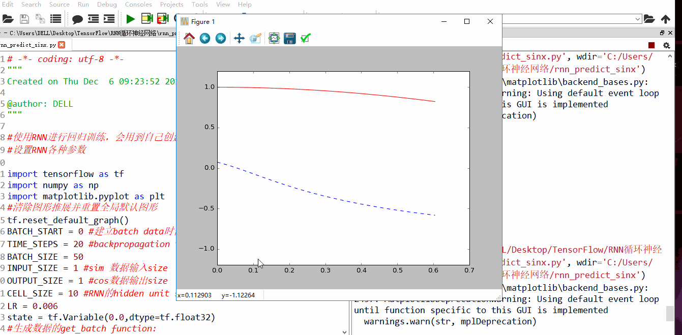
发现刚开始RNN蓝色曲线为预测去年,并不是很重合,随着慢慢的RNN训练,到60以后,预测曲线和实际曲线基本吻合。
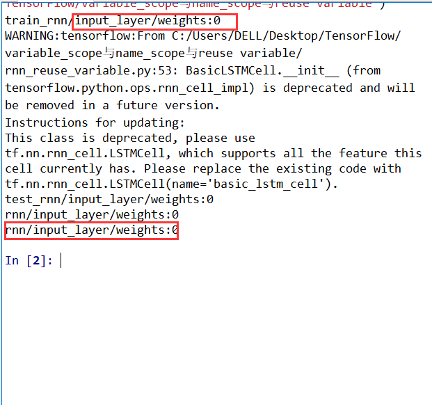
使用tensorboard
查看loss和graph
耗费了大量时间来讲解RNN和LSTM的原理,并且这一块确实有点难以理解。实践是检验真理的唯一标准,废话不多说,直接上基于TensorFlow平台的RNN加上LSTM优化后的代码和运行效果。
1 |
|
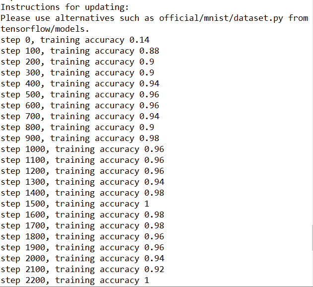
随着训练次数的增加,精确度也渐渐上升
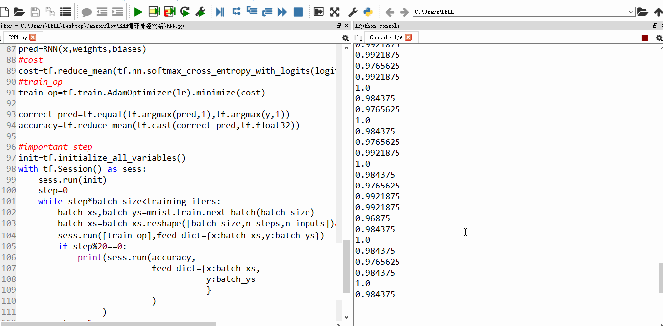
设置的训练100w次,每20步输出一次结果,由于时间太久,我就不一一截图了。训练结束后,精确度99%
一、LSTM结构
LSTM(Long-Short Term Memory),长短期记忆网络是RNN的一种变形结构。RNN因为梯度消失的原因只有短期记忆,LSTM网络通过精妙的Cell门控制将短期记忆与长期记忆结合起来,并在一定程度上解决了梯度消失的问题。
所有RNN都具有一种重复神经网络模块的链式形式。在标准的RNN中,重复的模块只有一个非常简单的结构,比如一个tanh层。
LSTM的结构:
LSTM同样的结构,但是重复的模块拥有一个不同的结构,不同于单一层,这里是由四个,以一种非常特殊的方式进行交互
二、LSTM的核心思想
LSTM有通过精心设计的称作为“门”的结构来去除或者增加信息到细胞状态的能力。门是一种让信息选择通过的方法。包含一个sigmoid神经网络层和一个按位的乘法操作
sigmoid层输出0~1之间的数值,描述每个部分有多少量可以通过。0代表不允许
任何量通过,1代表允许任意量通过。LSTM拥有三个门,来保护和控制细胞状态。
三、LSTM的推理
sigmoid层叫做输入门层,决定将要更新的值
tanh层创建一个新的候选值向量Ct,会被假如到状态中。
最后一步,确定需要输出什么值。这个输出将会基于我们的细胞状态,但是也是一个过滤后的版本。首先是,运行一个sigmoid层来确定细胞状态的哪个部分将被输出。然后,把细胞状态通过tanh进行处理,得到一个-1~1之间的值,将它和sigmoid门的输出相乘。
四、LSTM的变体
让门层也接受细胞状态的输入
使用coupled忘记和输入门
区别于标准LSTM的分开确定忘记什么和需要添加什么新的信息,变体的LSTM是两者一同做出决定。
RNN(Recurrent Neural Network)是一类用于处理序列数据的神经网络。序列数据:时间序列数据,也就是在不同时间点上收集到的数据,这类数据反映了某一事物、现象等随着时间变化的状态或者程度。也不一定是时间序列,也可以是文本序列。总之:后面的数据跟前面的数据是有关系,可以将RNN看做全连接网络
一、RNN的结构
普通神经网络包含input layer,hidden layer,output layer,通过Activation Function来控制输出。layer与layer通过weights连接。
两者区别:
基础的神经网络只在层与层之间建立了权Weights连接,RNN在层之间的神经元之间也建立了权连接
实际中,RNN标准结构并不能解决所有问题:
有时候输入时序列,但是不随着序列变化:
实际中,大部分问题序列都是不等长的。比如:自然语言处理中,源语言和目标语言的句子往往长度是不同的。就需要Encoder-Decoder模型,也叫Seq2Seq模型。
Encoder-Decoder模型结构原理:先编码后解码。左侧的RNN用来编码得到c,然后再用右侧的RNN把c解码。
二、标准RNN的流程
标准的RNN采用的是前向传播过程:
图中的:x为输入input,h为hidden layer单元,o为输出output,L为loss损失函数,y为training set训练集,右上角小标号代表t时刻状态。W,U,V代表权值Weights。
φ为激活函数,一般选择是tanh函数,b为biases偏置
t时刻的输出o:
预测输出为:
其中δ为激活函数,RNN常用语分类,这里一般用softmax函数
三、RNN的训练方法(Back Propagation Through Time,BPTT)
BPTT用来RNN训练。它的本质是BP算法,只是加上了时间。因为RNN处理时间序列数据,要基于时间反向传播。
核心思想:BPTT和BP算法相同,都沿着需要优化参数的负梯度方向不断寻找更优的点直到收敛。也就是梯度下降法。
需要寻找最优的有三个参数:U,V,W。
U,W两个参数的寻找最优的过程需要用到历史数据。而,V只关注当前h(hidden layer)的数据。
求V的偏导数**:**
也即是L(Loss)对V求偏导,V到L还经过o(output),里面有激活函数。所以是复合函数求导过程。
因为RNN的L(Loss)的损失是随着时间累加的,所以叠加后的结果如上图。
求W的偏导数:
W偏导求解需要用到历史数据,假设我们只有三个时刻,假设第三个时刻L对W的偏导数为:
求U的偏导数:
U偏导求解需要用到历史数据,假设我们只有三个时刻,假设第三个时刻L对U的偏导数为:
上面只是对某个时刻的W和U求的偏导数,但是RNN的L(Loss)损失是随着时间累加的,要追溯到历史数据,那么整个损失函数L对W,U的偏导数十分复杂的。通过找规律发现:
根据RNN图得知,Activation Function激活函数是嵌套在对h(hidden)的偏导里面的,把中间累乘部分替换为tanh或者sigmoid写法为:
上面的累乘会导致激活函数的累乘,会导致“梯度消失”和”梯度爆炸“现象。
1、sigmoid函数(logistics函数)和导数:
结论:使用sigmoid函数作为激活函数,肯定是累乘的时候结果越来越小,随着时间推移小数的累乘导致梯度小到接近于0,这就是“梯度消失”。梯度消失会导致,那一层的参数再也不会更新,那么那一层隐藏层就变成了单纯的映射层,就毫无意义了。
总结:sigmoid函数(logisitic函数)不是0中心对称
2、tanh函数和导数:
总结:tanh函数是中心对称,会导致神经网络的收敛性更好,是tanh函数相对于sigmoid函数来说梯度较大,收敛速度更快且引起梯度消失更慢
解决梯度消失的方法:
1、选取其他激活函数
一般选用ReLU作为激活函数
ReLU的导数:
总结:ReLU函数的左导数为0,右导数为1,避免了“梯度消失”,然而右导数为1,会导致“梯度爆炸”,但是可以设定合适的阈值可以解决“梯度爆炸”问题。还有一点就是,左导数恒为0,有可能导致把神经元学死,同样设置合适的步长(training_step)可以避免问题发生。
2、改变传播结构
改变传播结构,也就是引入LSTM(Long-Short Term Memory),长短期记忆网络。是一种时间递归神经网络。适合处理和预测时间序列中间隔和延迟相对较长的重要时间。LSTM区别于RNN的地方,就是在算法中加了一个判断信息有用与否的处理器Cell。
具体CNN的原理以及应用请看上一篇文章。废话不多说,直接上代码,看运行效果
1 | # -- coding: utf-8 -- |
Tensorboard的操作
利用Google Chrome查看图形化差异

1 | #author:victor |
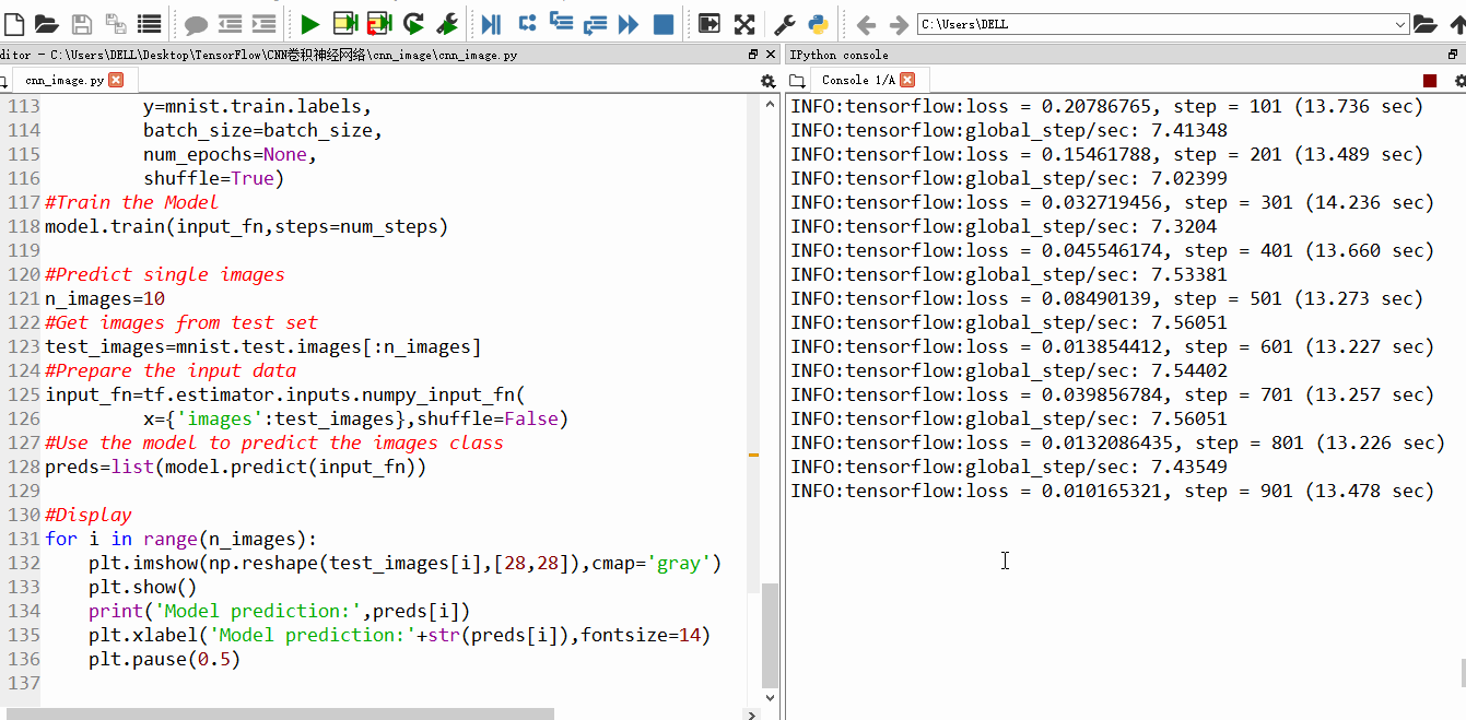
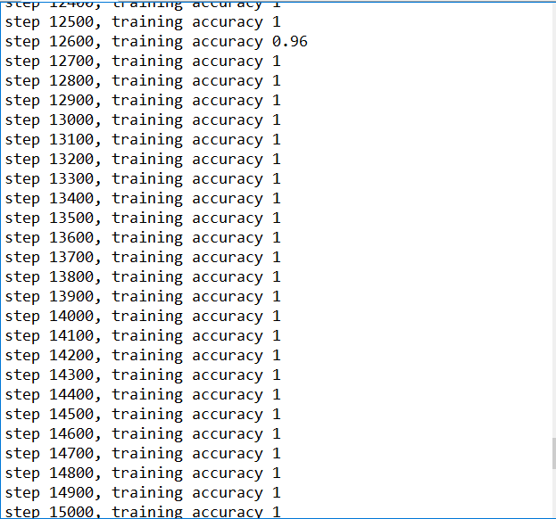
二、运行效果
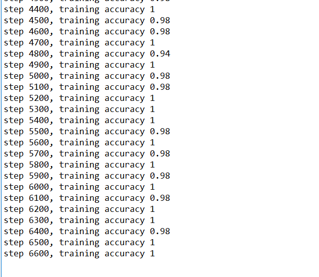
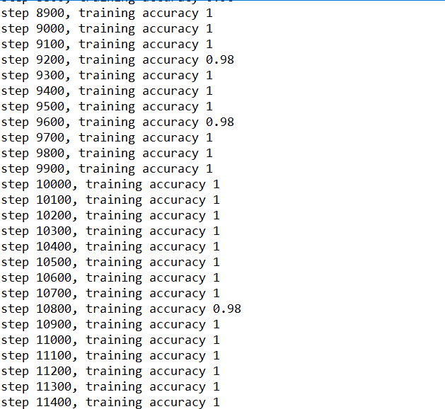
训练到15000步,精确度已经很高,几乎100%
训练结束后的结果
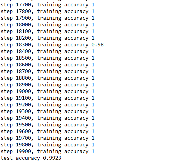
对比上一节的MNIST入门的Demo利用GradientDescentOptimizer直接进行训练,利用CNN训练,精确度基本上99%
ps:由于设置的循环range为20000,训练次数比较大,跑起来比较耗时,我安装的是CPU版本的Tensorflow,跑了大概1个小时训练结束。