线性回归(Linear Regression)
- 线性回归是利用数理统计中回归分析,来确定两种或两种以上变量间相互依赖的定量关系的一种统计分析方法,运用十分广泛。其表达形式为y = w’x+e,e为误差服从均值为0的正态分布
- 回归分析中,只包括一个自变量和一个因变量,且二者的关系可用一条直线近似表示,这种回归分析称为一元线性回归分析。如果回归分析中包括两个或两个以上的自变量,且因变量和自变量之间是线性关系,则称为多元线性回归分析。
- 梯度下降是用于找到函数最小值的一阶迭代优化算法。为了使用梯度下降找到函数的局部最小值,需要采用与当前点处函数的梯度(或近似梯度)的负值成比例的步长。相反,如果采用与梯度的正值成比例的步长,则接近该函数的局部最大值 ; 然后将该过程称为梯度上升。
废话不多说,直接上代码,展示运行效果
1 | #Linear Regression线性回归 |
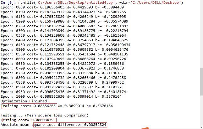
控制台的每一次梯度下降后的误差值:
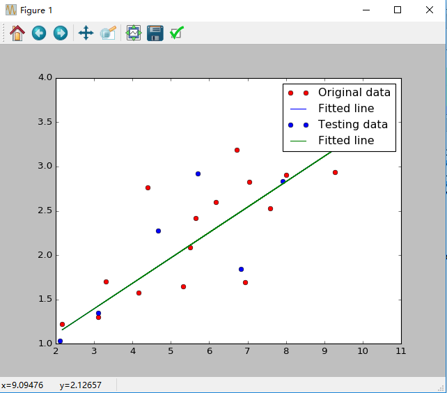
线性回归后的结果图展示: