
一、CNN的源代码
1 | #author:victor |
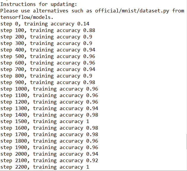
二、运行效果
- 刚开始训练精度并不高,在90%左右
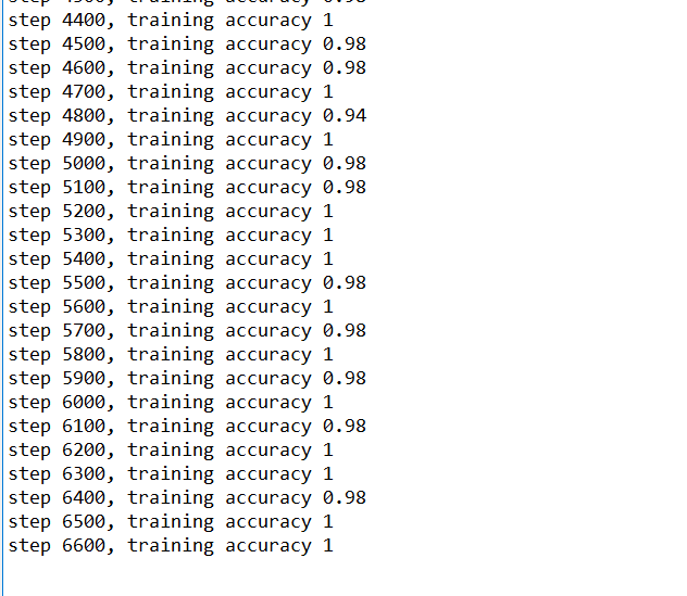
- 随着慢慢的训练5000步左右的时候,精度逐渐增加到99%左右
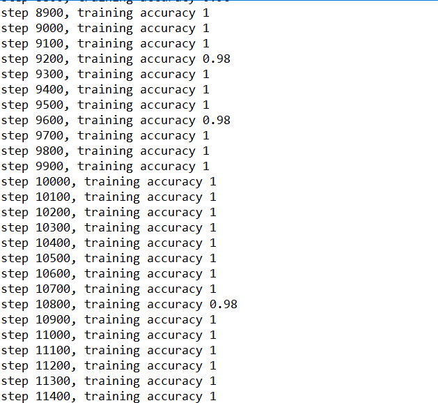
- 等过万的时候,精确度已经很高了,接近于100%
训练到15000步,精确度已经很高,几乎100%
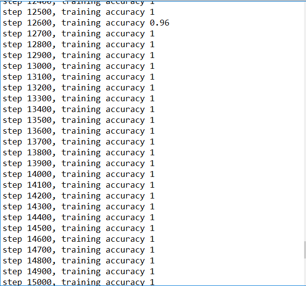
训练结束后的结果
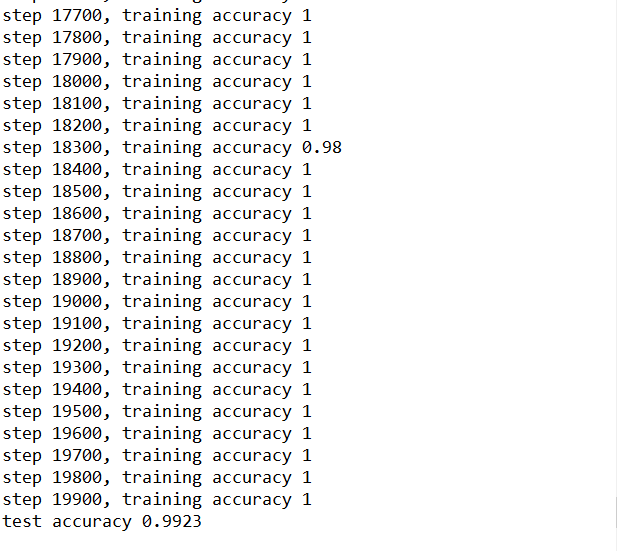
对比上一节的MNIST入门的Demo利用GradientDescentOptimizer直接进行训练,利用CNN训练,精确度基本上99%
ps:由于设置的循环range为20000,训练次数比较大,跑起来比较耗时,我安装的是CPU版本的Tensorflow,跑了大概1个小时训练结束。